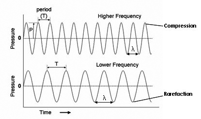
 The frequency of an ultrasound wave is above 20,000 Hz (or 20 KHz) and medical ultrasound commonly is in the 2.5-15 MHz range. Human hearing is in the 20-20,000 Hz range.
 Generation of an Ultrasound Wave
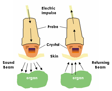
An ultrasound wave is generated when an electric field is applied to an array of piezoelectric crystals located on the transducer surface.
Electrical stimulation causes mechanical distortion of the crystals resulting in vibration and production of sound waves (i.e. mechanical energy).
The conversion of electrical to mechanical (sound) energy is called the converse piezoelectric effect (Gabriel Lippman 1881).
Each piezoelectric crystal produces an ultrasound wave. The summation of all waves generated by the piezoelectric crystals forms the ultrasound beam.
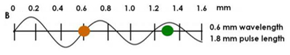
Ultrasound waves are generated in pulses (intermittent trains of pressure waves) and each pulse commonly consists of 2 or 3 sound cycles of the same frequency.
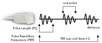
The pulse length (PL) is the distance traveled per pulse. Waves of short pulse lengths improve axial resolution for
ultrasound imaging. The PL cannot be reduced to less than 2 or 3 sound cycles by the damping materials within the transducer.
Pulse Repetition Frequency (PRF) is the rate of pulses emitted by the transducer (number of pulses per unit time).
Ultrasound pulses must be spaced with enough time between pulses to permit the sound to reach the target of interest and return to the
transducer before the next pulse is generated. The PRF for medical imaging ranges from 1-10 kHz. For example, if the PRF = 5 kHz and the time
between pulses is 0.2 msec, it will take 0.1 msec to reach the target and 0.1 msec to return to the transducer. This means the pulse will travel 15.4 cm
before the next pulse is emitted (1,540 m/sec x 0.1 msec = 0.154 m in 0.1 msec = 15.4 cm).

Advancing the Science of Ultrasound Guided Regional Anesthesia and Pain Medicine
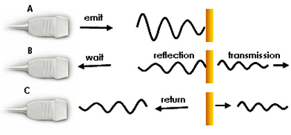
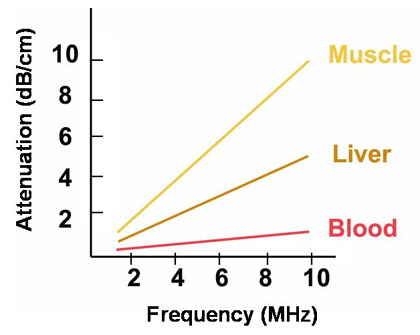 ↑ Frequency = ↑ Attenuation; ↑ Attenuation = ↓ Penetration
To compensate for attenuation, it is possible to amplify the signal intensity of the returning echo. The degree of receiver amplification is called the gain.
Increasing the gain will amplify only the returning signal and not the transmit signal. An increase in the overall gain will increase brightness of the entire image, including the
background noise. Preferably, the time gain compensation (TGC) is adjusted to selectively amplify the weaker signals returning from deeper structures.
↑ Frequency = ↑ Attenuation; ↑ Attenuation = ↓ Penetration
To compensate for attenuation, it is possible to amplify the signal intensity of the returning echo. The degree of receiver amplification is called the gain.
Increasing the gain will amplify only the returning signal and not the transmit signal. An increase in the overall gain will increase brightness of the entire image, including the
background noise. Preferably, the time gain compensation (TGC) is adjusted to selectively amplify the weaker signals returning from deeper structures.
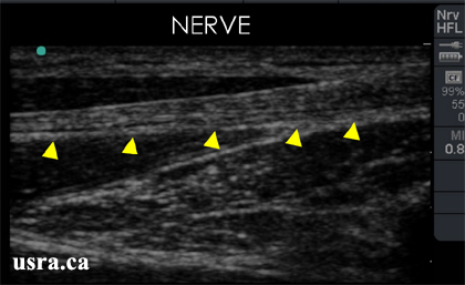 A nerve in longitudinal section (arrowheads) showing internal echotexture consisting of continuous hypoechoic longitudinal elements (fascicle groups) interspersed with hyperechoic perineural connective tissues.
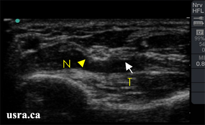
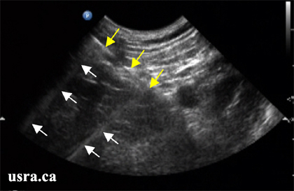
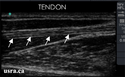 A tendon in longitudinal section (arrows); a tendon appears very much like a nerve in this view although the tendon has a fibrillar internal echotexture and discontinuous hyperechoic speckles.
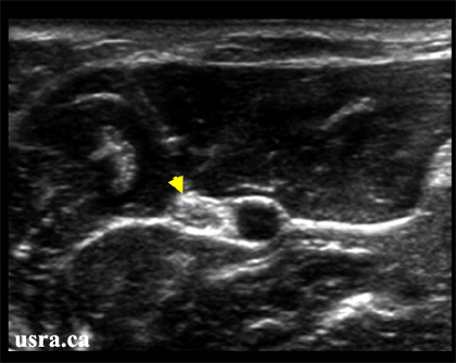
 A hypoechoic nerve root (arrowhead) in the low interscalene region; nerves are generally hypoechoic in the interscalene and supraclavicular regions; the hypoechoic component represents the neural tissue.
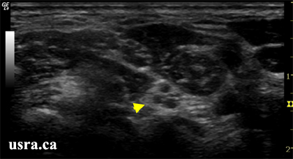
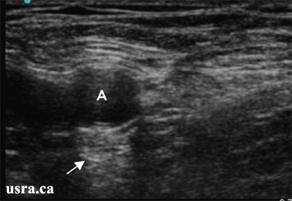
 Nerves below the clavicle and in the lower limbs are predominantly hyperechoic and have a honey comb appearance. For example, the median nerve in the elbow region
(arrowhead) is predominantly hyperechoic. The degree of hyperechogenicity likely reflects the amount of connective tissue within the nerve.
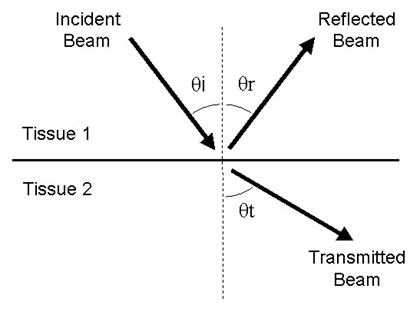
Anisotropy refers to a change in echogenicity of tissues (e.g., tendon and nerve) as a result of transducer angle. A hyperechoic nerve
structure can appear hypoechoic when the angle of incidence is changed from 90 degrees to 45 degrees (see
Nerves below the clavicle and in the lower limbs are predominantly hyperechoic and have a honey comb appearance. For example, the median nerve in the elbow region
(arrowhead) is predominantly hyperechoic. The degree of hyperechogenicity likely reflects the amount of connective tissue within the nerve.
Anisotropy refers to a change in echogenicity of tissues (e.g., tendon and nerve) as a result of transducer angle. A hyperechoic nerve
structure can appear hypoechoic when the angle of incidence is changed from 90 degrees to 45 degrees (see 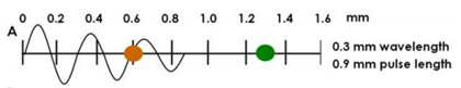
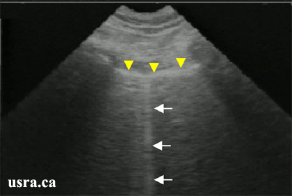
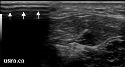 The air artifact (arrows) at the transducer skin interface is due to a lack of conductive gel and poor transducer to skin contact. This results in a large dropout artifact.